MC Escher, “Concentric Rinds” 1953.

I’ve since turned this code into a simple Shiny app that makes word clouds out of .txt files.

I recently came across the tidytext R package, and the accompanying book, Text Mining in R by David Robinson and Julia Silge. I found it very practical for basic text mining and NLP problems spanning tf, idf, tf-idf, word vectorization, cosine similarity, sentiment analysis, and topic modeling.

There are a pleathora of out-of-the-box functions and data that help with common natural language processing (NLP) tasks, like:

• tokenizing documents
• removing stop-words (e.g. - a, an, and, the, but)
• calculating tf, idf, and tf-idf

After playing around a bit with examples, I thought it would be interesting to see what the 38 page research prospectus I spent months slaving over boiled down to in terms of term frequency.

Bring in Data

I first saved my .docx file as a .txt in UTF-8 encoding because it’s easier for R to read. The result is a very messy table, which I won’t print here.

Load libraries and read data

library(dplyr) # for data wrangling
library(tidytext) # for NLP
library(stringr) # to deal with strings
library(wordcloud) # to render wordclouds
library(knitr) # for tables
library(tidyr)

# the local file path to my research prospectus
path <- '~/Documents/Github/rp/static/data/rp.txt' 

# fill = TRUE b/c rows are of unequal length
dat <- read.table(path, header = FALSE, fill = TRUE) 

1. Tidy

Since the package we’re using adheres to tidy data principles, step 1 is to get this messy table into a one column data frame, with one word in each row.

# reshape the .txt data frame into one column
tidy_dat <- tidyr::gather(dat, key, word) %>% select(word)

tidy_dat$word %>% length() # there are 10,480 tokens in my document

## [1] 10480

unique(tidy_dat$word) %>% length() # and of these, 2,866 are unique 

## [1] 2866

2. Tokenize

The next step is to tokenize, or boil the dataframe down down to only unique observations, and count the number of each observation. To perform this, we use unnest_tokens(), which takes 3 arguments:

• a tidy data frame
• name of the output column to be created
• name of the input column to be split into tokens

Then we use the count() function from dplyr to group by words and tally observations. Becauase count() performs a group_by() on the word column, we ungroup().

# tokenize
tokens <- tidy_dat %>% 
  unnest_tokens(word, word) %>% 
  count(word, sort = TRUE) %>% 
  ungroup()

Just because a token is common doesn’t mean it’s important. For instance, take a look at the most 10 common tokens in my research prospectus.

tokens %>% head(10)

##           word   n
## 1          the 487
## 2          and 368
## 3           of 344
## 4           in 235
## 5           to 235
## 6  groundwater 193
## 7        water 138
## 8            a 137
## 9           is 112
## 10         for  92

Of the 10, only 2 actually tell us something about what’s written about: groundwater, and water. Cleaning natural language is like panning for gold: most of language is useless, but every once in a while we find a gold nugget. We want to get only the nuggets.

3. Remove Stop Words, Numbers, Etc.

tidytext has some built-in libraries of stop words. We’ll use an anti_join() to get rid of stop words anc clean our tokens.

# remove stop words
data("stop_words")
tokens_clean <- tokens %>%
  anti_join(stop_words)

## Joining, by = "word"

While we’re at it, we’ll use a regex to clean all numbers.

# remove numbers
nums <- tokens_clean %>% filter(str_detect(word, "^[0-9]")) %>% select(word) %>% unique()

tokens_clean <- tokens_clean %>% 
  anti_join(nums, by = "word")

I also did a quick pass over tokens_clean to look for other meaningless tokens that escaped the stop-word dictionary and the numbers. It’s not surprising that the tokens that made it by were:

• al - from citations (e.g. - et. al)
• figure - figure captions and references in my prospectus
• i.e. - gotta love those parentheticals
• etc…

I’ll store these unique stop words in a vector and perform another anti_join, et voila. A tidy, clean list of tokens and counts.

# remove unique stop words that snuck in there
uni_sw <- data.frame(word = c("al","figure","i.e", "l3"))

tokens_clean <- tokens_clean %>% 
  anti_join(uni_sw, by = "word")

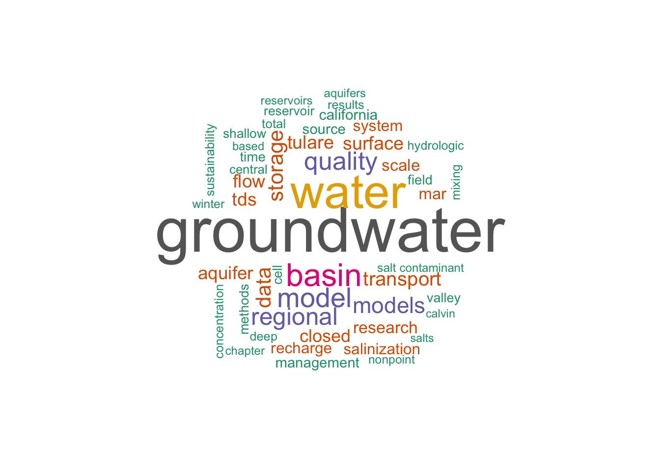
4. Make a Word Cloud of the top 50 words

And just like that, an easy word cloud. In fact, this code was so simple and fun that I wrapped it into a Shiny App.

# define a nice color palette
pal <- brewer.pal(8,"Dark2")

# plot the 50 most common words
tokens_clean %>% 
  with(wordcloud(word, n, random.order = FALSE, max.words = 50, colors=pal))